Introduction
It has been known for a some time that the spectrogram of the audio from obelisks found in Guardian Ancient Ruins [1] exhibits a series patterns comprised of vertical bars. Ever since the phenomenon was discovered [2], many have referred to these patterns as “barcodes” because of their resemblance to an ancient Earth technique of storing information in successive vertical bars. Many have attempted to decode these patterns, which we will refer to as data packets in this analysis, but have yet to see any underlying meaning, namely because no repetition in the stream of data packets has ever been observed. Even the most extensive documented analysis did not see a single repetition in 4 hours of audio [3].
Many have therefore despaired and concluded that the phenomenon is nothing but procedural gibberish, i.e. random patterns with no real underlying meaning. But such explanation is not satisfactory to this author. There could be a number of reasons why we have not been able to decode the obelisk data packets. For one, it is possible that each of the packets is part of a very long list of items, which would explain why no data packet had been observed twice. All efforts thus far might only be catching a snippet of the full list of items. Another reason why it has been hard to decipher the patterns is that there hasn’t been an adequate physical or mathematical quantity to which we can correlate these patterns with. There are many different possible quantities that these data packets could correlate with, the sheer number makes it a challenging task.
With the above considerations in mind, in this analysis we postulate the following hypothesis:
Each data packet represents the distance to another obelisk elsewhere in the galaxy.
This would explain why the list of items is so long. It is commonly accepted that there could be many more hundreds, if not thousands, of other sites throughout the galaxy, each of which contains a plurality of obelisks (indeed, new Ancient Ruins are being discovered to this day). The hypothesis above also gives us something else to work with: we can try to decode the data packets by correlating them to distances between obelisks at different sites. We don’t have to wait for the full list of items to cycle over in order to begin an attempt decode the patterns in the data packets.
Nevertheless, it would be highly encouraging to see a repetition of a data packet, in any capacity. In this analysis we will therefore collect lots of audio data and then *efficiently* process that data in order to 1) try to catch a repetition, 2) carry out a full characterization of the data packets and their statistics in order to have a good chance at decoding them. An Automatic Data Packet Recognition (ADPR) algorithm was developed to automatically extract and save the patterns observed in the obelisk audio spectrograms.
Data Acquisition
The GS164 Ancient Ruin site was picked because of its proximity to the derelict megaship The Cete [4]. It should be noted, however, that the presence of the The Cete does not have any bearing on this analysis (scrutiny of that megaship might be the subject of another article, but we can say right now that no clues were found there). Within the GS164 site the O03 obelisk was picked because it was far away from other active obelisks, thereby eliminating the chance of audio cross-contamination.
An SRV was parked right in front of the glowing segment of the obelisk. The hand break was engaged to ensure no motion was introduced into the experiment. Audio from the obelisk was captured using the Audacity software at a sampling rate of 44100 Hz in a single channel (mono), which is more than sufficient to capture the high frequency component of the obelisk audio. The audio was recorded in one hour segments. Since there can be several minutes of silence between data packets, it was not an issue to commit the recording to storage and restart another. Additionally, the refueling of the SRV was carried out during these breaks.
Two contiguous data taking sessions were carried out, one lasting 12 hours and the second one 9, for a total of 21 hours. This yielded 558 data packets. Due to a couple of refueling mishaps, two data packets were lost as a result of system audio contamination (that’s when we learned the value of premium fuel).
[note: we did not have the Ram Tah mission and the obelisk was never scanned.]The Anatomy of a Data Packet
The figure below shows the components of an obelisk data packet, which is divided into two segments: the sequence of bars that comprise the main segment of the packet and the end-of-packet sequence. The main segment of the packet, the one that seems to actually carry information, is composed of a combination of the following vertical bars:
- Long bars that occupy the majority of the frequency range and have a duration of 0.66 seconds. In this study these will be denoted with the letter L.
- Short bars that roughly occupy the upper half of the frequency range and have duration of 0.75 seconds. In this study these will be denoted with the letter S.
- Thick bars that roughly occupy the lower half of the frequency range and have a duration of 1.66 seconds. In this study these will be denoted with the letter T.
- Narrow bars that occupy the full frequency range and have duration of 0.25 seconds. In this study these will be denoted with the letter T.

The data packet is capped by an end-of-packet sequence comprised of a narrow bar, some sparse spaces (explained in a bit), and a wide “end” bar that occupies the full frequency range; the latter is denoted as E in this study. The end-of-packet segment is 12.460 seconds from the left edge of the N bar to the right edge of the E bar.
The sparse spaces–named as such because they are not actually empty and tend to have 7 horizontal lines at various frequency values–come in 12 varieties, 5 of which can only be found in the end-of-packet segment between the N and E bars. A summary of the vertical bars and the sparse spaces in given in the table below along with their corresponding IDs. This naming convention was chosen for its descriptive simplicity and ease of use.
It should be noted that sparse space 6 is always found to the right of N bars in the main packet sequence. Sparse space 12 is always found to the left of L bars.
[editorial note: It turns out that 10 and 6 are the same, didn’t notice on first pass of analysis.]
Automatic Data Packet Recognition (ADPR) Algorithm
In addition to spending hours to collect audio data, one can spend even longer periods of time extracting the data packets. Such onerous activity can break the will of even the most committed of scientists. In order to meet this challenge, a special algorithm was developed to automatically extract the data packets in an efficient manner. In addition to retrieving the correct designation of each bar, the algorithm also captures the time differential between all of the components of the data packet.
A series of conceptually simple (but not so easy to implement) heuristic techniques were used to differentiate and extract the data packet components from the surrounding noise. Information such as the fact that N and L bars always have adjacent sparse spaces was leveraged to help disentangle the signal from the noise. For the sake of brevity, the low-level details of the algorithm will not be discussed here. The figure below shows a high-level overview of the algorithm.

As described in the data acquisition section, audio data is collected in one hour chunks. Due to memory limitations, these one hour chucks are sub-divided into segments roughly 15 minutes long. Each of these 15 minute segments is the input to the ADPR algorithm.
The first step is to form the spectrogram. This is achieved with a spectral slice of 5 milliseconds and an FFT size of 512, which is sufficient to carry out detailed frequency selection. A rough bandpass filter is applied to limit the frequency range between 9.5 and 16.5 kHz, the area where the data packets live. The algorithm then proceeds to find the packet edges by detecting E bars.
For each of the data packets, the algorithm uses a divide and conquer approach to detect the signal components of the main packet segment. It starts with the easiest, most prominent bars and works its way to the most difficult ones. The T bars are the easiest to detect because they are the widest (in the main segment), but for technical reasons the algorithm begins with the S bars. After detecting the S bars, they are masked out (i.e. disregarded downstream) in order to minimize false alarms. This process is repeated for the T, L, and N bars respectively. The designation and relative time location of each bar is saved for later analysis.
It should be noted that the probability of correct detection is in the high 90’s for each of the bars. False alarms associated with N bars tend to pop up here and there, but thankfully these don’t happen very often and are easily removed manually.
The figure below shows a processed data packet. The detected bars are indicated by the dashed squares. The end-of-packet segment is indicated by the large box on the right. The full code of this data packet is LTLSNNE. All data packets end with the NE designation because those are the only two bars associated with the end-of-packet segment.

The figure below shows a more complicated data packet, with a code that reads LSSLSTSTLTNSSLTLLSTLSNNE.

Data Packet Statistics
The first order of business was to check if the data packet stream exhibits any sort of repetition. No general repetition pattern was observed in the 21 hours of data collection. However, of the 558 extracted data packets, 3 pairs have the same sequence of bars, albeit with differences in the spacing between adjacent bars. Since we don’t yet know if the sparse and blank spaces convey information, we can’t conclude with 100% certainty that we have seen observed the same data packet twice. (note: a new data collection was carried out in GS001 that is not included in this analysis. That data collection confirmed 6 more additional pairs. Those results will be included in a future analysis).
The figures below show a comparison of the 3 data packets and their corresponding repetitions. The first figure shows a comparison of two data packets with the LLNSTNE pattern. The spacing differences between the bars in the two data packets is evident. The same can be said of the other figures comparing patterns TSNSTLNE and SLTLTNNE, respectively, though it must be noted that out of the three the SLTLTNNE pair show the closest resemblance to one another.


This begs the question, are the sparse spaces significant? Do they convey information? If that’s the case, then we are not seeing the same pairs of data packets with the same underlying information. It’s very probable that the sparse spaces are significant, otherwise why not just have a neat row of evenly spaced bars? With that in mind, we now turn to the topic of the statistics of inter-bar spacings.
The figure below shows a histogram of the spacing between adjacent S bars. The pattern is symmetric because of the obvious symmetry of left-to-right versus right-to-left. To be clear, the spacing shown in the figure corresponds to the left-edge to left-edge distance (it is admittedly somewhat counter intuitive to plot it this way, but we found the differences are easier to see in this manner). The negative side of the horizontal axis corresponds to the left side distance and the positive to the right side distance. The first thing to note here is the apparent grouping of the statistics: 1) S bars don’t like having arbitrary spacing between each other, 2) the separation is almost quantized, with three major groups, 3) S bars require a minimum of 1.25 seconds of spacing between each other (after taking into account their widths). It was observed that one or more of the sparse spaces intervenes between the two, almost as if “like bars/charges repel”.

The figure below shows the spacing between S bars and all other bars. A similar quantization pattern is evident. A detailed breakdown of each of the groupings shows that they correspond to each of the other bars. The slight asymmetry in the histogram is due to the fact that L bars and N bars always have adjacent sparse spaces, as discussed in a previous section.

The same type of behavior is exhibited by the statistics of the other bars (for the sake of brevity they will not be shown): L bars require a minimum of 1.59 seconds between each other, N bars require 2.25 seconds, and T bars require 1.34 seconds (after taking into account their widths). In the case of N and L bars, part of the minimum distance is due to the sparse spaces they always have attached. We are still in the process of investigating the statistics of the sparse spaces that fill the area between like-bars. Needless to say, the observed spacing patterns will place a significant constraint on whatever numerical system is derived from the overall patterns in these data packets.
We now turn to the statistics associated with total packet length, as measured by the number of bars/digits in each data packet (this includes the NE in the end-of-packet segment). The figure below shows a histogram of data packet length. There are a number of interesting features in the distribution:
- the minimum packet length observed is 6
- the maximum packet length observed is 45
- the distribution is NOT flat. It has a peak value at length 9, a secondary peak at length 16, and tapers off rapidly with increasing length.

The packet length distribution with a distinct structure is quite possibly the most profound result of this analysis. While it is very possible to “dial in” an arbitrary probability distribution function (PDF) that generates random bar lengths, why would the PDF have the distinct structure we see? Why not a something like a flat PDF? Why not a PDF that is more reflective of the total possible number of N-L-S-T combinations for a given packet length (minus the end-of-packet segment)? (in that case, the PDF would be overwhelmingly biased toward longer packet lengths).
The distribution above looks like it wants to be a Poisson distribution, but then why do we see that second peak? Sure, the fde…, er, The Guardians can dial in whatever they want, but why this particular shape? The distribution above is probably the best piece of evidence that we have supporting the idea that these data packets might actually correlate with something we can measure and not just a random phenomenon. Or we could be looking at a combination of garbage information (accounts receivable, number of Guardian biscuits delivered across the galaxy, etc.) and meaningful data.
Having said that, it should be noted that two additional observations stick out: 1) All of the data packets collected in this study exhibit at least one of each of the four types of bars, 2) We have yet to observe a data packet with a length of less than 6, i.e. with a main segment comprised of less than 4 bars. The latter could be the result of the packet length PDF having a vanishingly low value for lengths less than 6, or alternatively it could be that the information carried by these data packets correlates with physical quantities that require a minimum number of digits/bars (such as distance to another system). The first observation might also constrain whatever numerical system we can derive from the patterns in the data packets.
It should be noted that, in terms of overall counts, each type of main segment bar was observed around 1850 times among the 558 data packets collected. There are slight variations among the bars, but these are within statistical uncertainties given the sample size.
Cursory Attempt at Correlating Data Packets with Distances
Since we are having trouble seeing repetitions in the stream of data packets, one thing we can do is to try to decode the data by correlating it with a physical quantity. Several researchers in the community have brought up the idea of mapping the sequence of bars to quaternary encoding. The main focus of this analysis was to characterize the global properties of obelisk data packets, but nevertheless in this section we give it a quick shot.
If we assume that each of the four bars maps to a value of 0, 1, 2, or 3, then we can extract a value out of a sequence of bars (we’ll be ignoring sparse spaces for now). There are 24 possible ways you can do such a mapping [5]. For each one we tried to correlate all of the collected data packets to the distance between the GS164 system and all other known systems with Ancient Ruins. The hope was that one of the combinations would prove to be the correct by having many more “hits” than the other combinations. In order for a match to be declared, the difference in distance values between a given data packet and particular system must be less than 2 Ly.
The table below shows the number of hits for a each of the 24 possible mappings. The number of hits varies between 7 and 12, but none exhibit an obvious spike in hits. There are many other possible ways to map the data packet patterns to numerical systems, even ways that incorporate the sparse spaces into the system. Other ideas will be tried in the future.

Summary and (Preliminary) Conclusions
An algorithm was developed to sift through 21 hours of obelisk audio containing 558 data packets. A number of interesting observations were made about the way the bars in the main segment of a data packet are arranged, namely a minimum spacing of at least 1.25 seconds between adjacent bars of the same type. All observed data packets contain at least one of each of the four bar types.
Only three data packets were observed to repeat, but with some differences in the spacings between adjacent bars. We have yet to see two data packets that look exactly the same.
The most striking result in this analysis is in the distribution of packet lengths, which has a particular structure not consistent with the usual PDFs associated with random processes, such as flat, Poisson, or Gaussian PDF. This could mean that (at least a portion of) the data packets might correlate to a physical quantity.
The next step in this avenue of research is to collect data at other sites around the galaxy, preferably far away from the Col 173 Sector bubble in order to see how the distribution of packet lengths changes. If it stays the same, then we’re probably looking at data packets that carry random information.
References
[1] Mykl Atrum, “The Guardians”, https://canonn.science/codex/the-guardians/[2] CMDR Ericlas, “Obelisks transmitting Binary/Morse/…/just random noise ?”, https://forums.frontier.co.uk/threads/alien-archeology-and-other-mysteries-thread-9-the-canonn.300054/page-301#post-4751754
[3] CMDR stick152, “Some Thoughts on Obelisk Audio”, https://forums.frontier.co.uk/threads/alien-archeology-and-other-mysteries-thread-9-the-canonn.300054/page-335#post-4765655
[4] CMDR Scott (Keybuck), “The Cete”, https://canonn.science/codex/the-cete/
[5] Math Planet, “Permutations and Combinations”, https://www.mathplanet.com/education…d-combinations